利用者:Phonybone/Archive/ParticlesDesign/Components/Animation

Animation

Animation in a broader sense means defining how the particle system state changes over time. This can be done in two different ways (both methods described in detail below):

• Simulation makes incremental changes to the state.
• Caching can load states from a cache file or memory, if they were previously stored.

In general caching has preference over simulation stepping. This means that if a valid cache state can be loaded for the new frame, that will be used (see Caching for a definition of valid cache state).

Note: This follows these guidelines for physics systems.

Simulation

Simulation means calculating a new state by incrementing from the current frame/time.

Time Step

Incremental simulation generally works only for positive frame steps, i.e. simulation can not be "run backwards" (Note: individual elements, such as newtonian physics or keyframe animation may still use reverse timing, but this is an internal feature).

The frame step should always be broken down into steps of at most one frame at a time. This ensures that the simulation result does not depend on the total size of the frame step, for example when skipping multiple frames or scrubbing on the timeline.

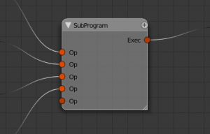
The simulation system must generally support subframes. This means that the frame step can be broken down further into fractions of a full frame and calculate intermediate results for each subframe. This is an important way of increasing accuracy and stability for many physical simulations and avoid visual artifacts. To allow a little more fine-grained control over which parts of the simulation need more subframes, a "sub-program" node can have a "frame divide" number. The sub-program would then execute its operator sequence multiple times with subframe steps divided accordingly (see Simulation Nodes for the concept of program nodes).

Simulation Nodes

There are so many different ways to achieve a specific result that it is impractical to perform simulations by just a couple of different fixed algorithms or even a bunch of "black boxes" (modifier stack), that can only be controlled by a handful of parameters.

As a solution to this problem node systems have proven to be immensely valuable. Most other 3D softwares offer much more advanced node configurations by now than what Blender has to offer. So as a first step a comparison of the two well-established programs Houdini and XSI/Softimage has been undertaken, the results of which can be found here: Houdini vs. XSI

While both systems have their pros and cons, Blender's current nodes were designed with ICE (XSI) in mind. This means that with just a few additional features, the node system can reach the required flexibility.

1. Extension of the node tree execution process with operator sockets (control structures and sub-programs)
2. Access to external data with get/set nodes.
3. Implementation of generic data context on sockets

Control structures

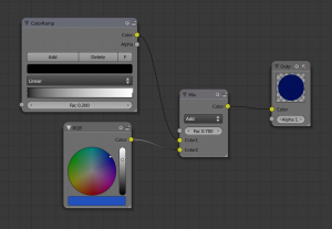
In terms of programming the current node trees basically describe one large expression. Each node can be seen as a set of functions (each output is the return value of a function), sharing the same parameter set from the input sockets. The outmost function is the output node, with each input being a nested function expression itself. For performance reasons the intermediate results are stored and re-used if a node is used as a parameter several times (i.e. has an output linked to multiple inputs). This kind of node tree is sufficient for shading or compositing where the task is just to produce a couple of colour/depth/etc. values for output.

Example node tree

Pseudo code of the expression:

Output(
    Add(            // "Add" node on Color input
        ColorRamp(
            0.2     // Fac default input
        ),
        RGB()
    ),
    1.0             // Alpha default input
)

Shader/texture/compositor nodes simply generate a value and leave the actual modification (of the render result) to code outside the node tree. Simulations are a different deal: they are supposed to modify the scene data by itself, i.e. many simulation nodes actually operate on scene data instead of just the local values (see Data Access Nodes below).

The consequence is that a more explicit way of executing nodes in a simulation tree is needed. Current "data nodes" are still an important part of the node tree, but rather than executing the whole tree one time calculating data for one (or several) output nodes, parts of the tree can be executed on their own. Another way to look at it is assembling a simulation tree from smaller sub-trees, each of which has it's own "output" in the form of an operator node.

Executable operator nodes would not be of much use without the introduction of control structures. These nodes reproduce some of the standards known from programming languages:

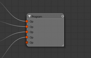
• (Sub-)Programs: Execute a list of other operator nodes in a sequence.
• "For" loops: Execute an operator node a given number of times.
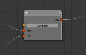
• "If" conditionals: Execute one of two branches according to a condition.
• Switch: Execute one of several branches according to an integer/enum input.

Operator nodes are integrated into the tree in the same way as regular nodes by the use of operator sockets. These are a new type of socket, which has no data associated to it, but denotes the use of an operator node by the target: The target node will use that operator when executing the socket. See the examples below.

Central output node with an extensible operator input list.

Subprograms have an additional operator output.

Only one of the branches is executed.

The input operator is executed several times.

An important thing to note here is that each node should have only one output operator socket. This is not strictly necessary in a technical sense (a node could be executed in different ways), but it helps keeping the design clean: What a node does when being executed should be clear from its type. If a there are several different things one could do, it should be different operators, i.e. different nodes, instead of squeezing two functionalities into the same node.

Data Access Nodes

Data access is naturally divided into two parts: Get and Set.

Getting data from the scene into the node tree has always be a part of the node trees (though in a rather limited form):

• Material nodes provide access to material settings.
• Geometry node provides a selection of commonly used shader input.
• Render layers feed render data into the compositor.
• etc.

Input to the simulation tree works pretty much the same way, but the range of data input types desirable is much greater. Most important input is of course the particle data. A particle simulation however does not make much sense without access to other objects (especially meshes), materials and textures.

The output of current node trees is a very limited and clearly defined set of colors and vectors (or pixel buffers respectively). Simulation nodes on the other hand do not have any predefined output data - they operate on the particle data (or any other scene data if we take this a step further). Therefore it is not sufficient to have an output node, which simply hands a few values over to the caller of the node tree for applying to the scene data or render result. Instead a generic counterpart to the GetData node(s) in the form of a SetData node is required. The SetData node has to make sure to update the scene data in a reliable way, which means that it has to update the dependency graph.

Data Collections and Context

Many elements in a simulation are actually collections of components:

• Particles
• Mesh vertices, edges and faces
• Images pixels

When a part of the node tree makes use of any property of such a data element (e.g. the particle position, vertex color, etc.), it actually has to be executed for each element in the collection. This causes some difficult situations regarding the execution process of the tree, especially when different collections are combined or nodes require intermediate results. Here are some examples:

• Multiplying a component property by a constant factor (which is not part of the collection)
• Adding two vectors from the same collection (e.g. calculating the average of two particle vectors 0.5*(a + b)).
• Filtering a collection: only a part of the elements is used by the nodes on the output side.
• Calculating the sum of all values in the collection. The node has to iterate over each element in the collection before the result can be used by following nodes.
• Normalizing a collection, i.e. dividing by the maximum element. In contrast to the calculation of average value above, this produces the same collection on the output side, but still has to iterate over all elements to find the maximum.

The one thing you will not find in these examples is the combination of different collections: The actual set on which such a node should operate is ambiguous and it's size can quickly go to extremes (it is basically O(n^2)), which is why combining elements from different collections is generally not allowed. For example you can not

• Add positions from different particle subsets
• Set the vertex color to faces (there are usually less faces than vertices in a mesh)

In order to allow nodes to process collections, it is necessary to give them information about the context of their input data. Each output socket defines a context (if it is part of a collection), which contains information about the source of elements and how to initialize and advance a collection iterator.

to be continued ...