Dev:Source/Modeling/Bevel
Bevel
These are developer notes about the Bevel algorithm in Blender.
Note: some discussion of user opinions about Bevel are here.
Edge Bevel: Requirements
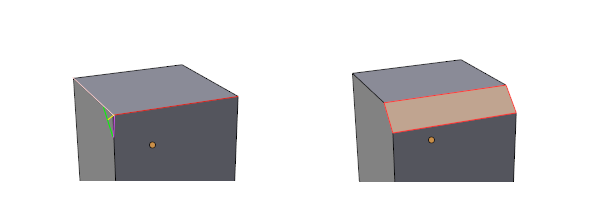
If you have an edge that is part of exactly two faces, an edge bevel should replace that edge with two parallel edges, each moved some distance along their respective faces. Usually the distance moved along each face is the same.
Bevel Amount
In the Bevel Edge figure the red edge is beveled. Four different ways of measuring the bevel amount are shown by colored lines on the diagram on the left:
- Offset (magenta line) - the distance each line moves on its respective face
- Width (green line) - the distance across the newly made face between the two lines
- Depth (yellow line) - the distance from the old edge to the new face, along the line that bisects the angle between the two faces
- Percentage (percentage of pink line) - the distance moved along each face is a percentage of the edge along which the new edge endpoint slides
Note that the Percentage case is strange in several ways: because it moves each of the 4 endpoints of the two new lines a distance that depends on the length of an adjacent edge, the resulting new edges may not be parallel, and the distance that the two lines move along their respective faces may not be the same. Some users have asked for this as an option, however, in order to create special modeling effects (there's an airplane wing modeling tutorial that uses it, for example).
When beveling a single edge, the first three methods are equivalent in that they all produce the same final models, just with different actual values of bevel amount. For a given final result, the amounts are related to each other by simple trigonometric functions of the angle between the faces. The current Bevel in Blender uses the Offset method for measuring bevel amount, by default.
However when beveling more than one edge at once, on a model that isn't completely symmetrical and with 90 degree angles, the different measurement methods yield different results.
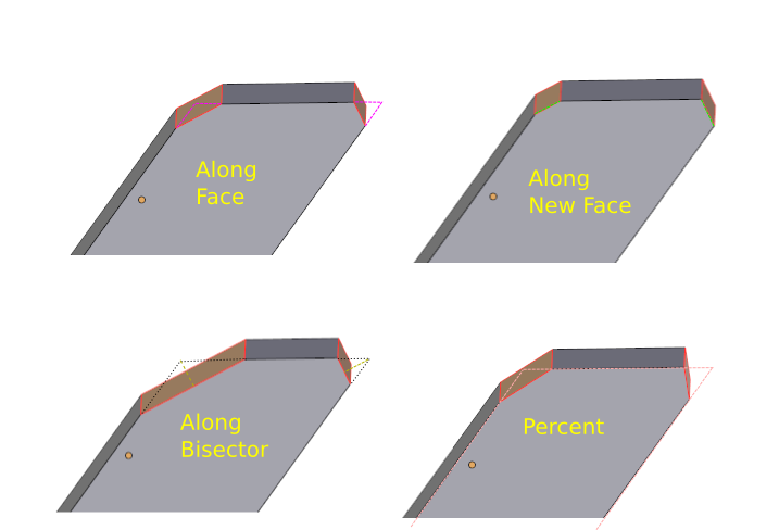
In the Bevel Offset Methods figure, you can see the effect of using the same offset but different offset methods on faces that meet in obtuse or acute angles. The same colors as in the Bevel Edge figure show where the specified distance (the same here for all methods except percentage) is measured. For the percentage case, the size and shape of the offset depends on how long the face is in the direction away from the beveled edge.
From the above diagram, it looks like the Width method gives more even looking results. However, when you bevel all edges around a face, and all around a vertex, the Offset method has advantages.
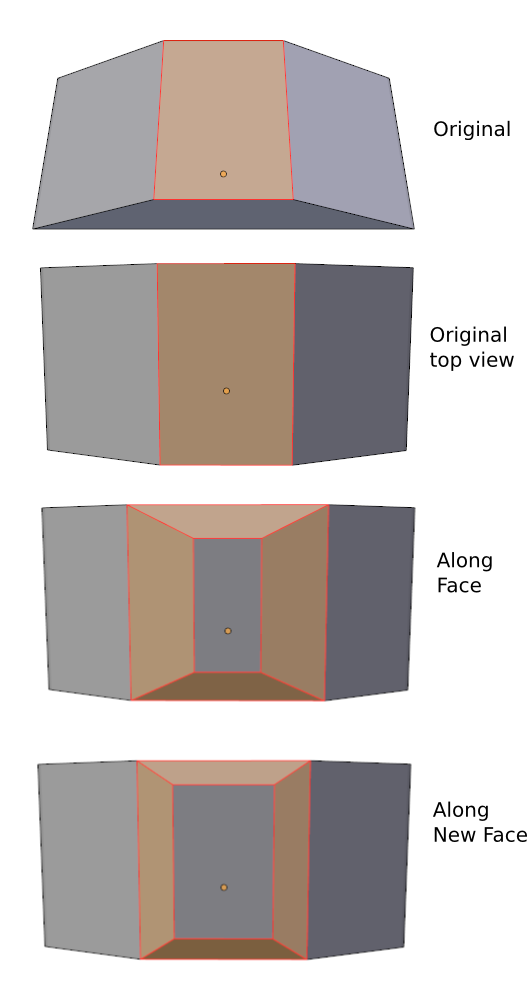
Notice that in Bevel Offset Methods On Face figure, the Offset method results in a new inside face that has a similar shape to the original face. This is because it insets each edge the same amount. Whereas the Width method has a different shape from the original face because each edge moves in a different amount, depending on the angle between the top face and the face on the other side of the beveled edge.
Probably artists would like the option of either Offset or Width. The argument for Depth is more theoretical: it corresponds to the physical act of planing of the edge and going to the same planing depth on each edge. That might make sense to some artists, though in practice it doesn't seem very useful. The Percentage method, as mentioned above, seems to have specialized uses that some artists want sometimes.
Non-manifold Edges
What to do about beveling edges that are non-manifold - that is, they are not connected to exactly two faces? For example, an edge that is the outer boundary of a plane, or an edge where three or more planes meet in a kind of fan. While one can imagine things to do in these cases, for now the decision in Blender is to regard Edge Bevel as only working on manifold edges. Non-manifold edges will be ignored when beveling.
Beveled Edge Ends
It is not always clear how to finish off the ends of beveled edges.
One case where it is pretty clear is when the vertex at the end of the edge is on an outside boundary, so the only two faces involved are the faces adjacent to the edge.
At a vertex where three edges meet, with three faces between them, and only one edge is beveled, most people would expect the result on the left in the next figure. But the result on the right is another option.
In the left result, the faces between the non-beveled edges are carved away by the end of the beveled edge. In the right result, those faces are instead split by the ends of the beveled edge. Let us call the left method Vertex Deletion and the right method Vertex Preservation, where this refers to whether the vertex at the end of the original beveled edge is removed from the final result or not. One could make these two choices an option, but in situations like this Vertex Perservation doesn't seem very useful, so for now Blender will always use Vertex Deletion in this one-of-three-edges-beveled case.
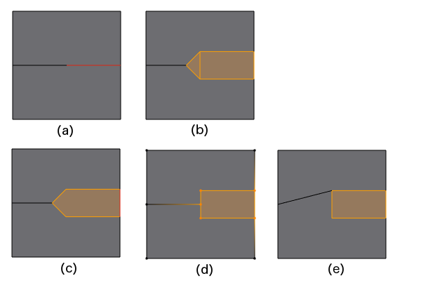
A vertex where only two edges meet and only one of the edges is beveled presents another problem.
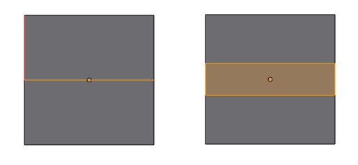
In the figure above, (a) is the original, showing a split edge in a plane, and (b) - (e) show four choices of how to end the bevel. Of these choices, only (b) and (e) make a new bevel face that is a quad, something that seems desirable. Also, choices (c), (d), and (e) will make non-planar ngons if the upper and lower faces in (a) are not coplanar. Blender currently always uses choice (b) for situations like this.
Even with choice (b) there is another subchoice to be made: what size angle should we make at that triangle tip (or, equivalently, how far along the unbeveled edge should we slide to get the position of the new end of that edge)? The current choice is to slide it by the offset (the Offset distance, see above).
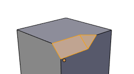
In the nonplanar case, this may not be exactly what is desired:
An artist might like the option to specify the slide distance as zero in this case, to make a nice vertical transition between the beveled and unbeveled edges.
Now consider the case of more than edges into a vertex, all beveled.
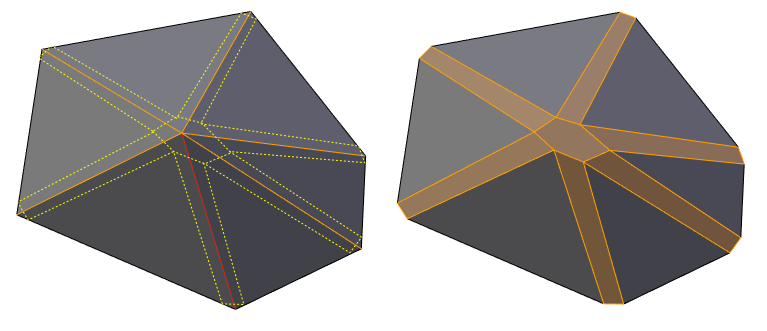
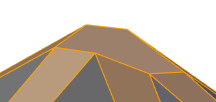
In this figure, where all six side edges of an irregular six-sided cone are beveled, it is pretty clear what to do. On the left side you see the original mesh, with dotted yellow lines showing the construction of the bevel. Whichever way the bevel amount is specified by the user, that can be translated into the Offset amount for each edge. Even if two adjacent bevel edges have different offsets, as they will in general when anything but the Width method has been used, there is always an intersection point on the common face. The old vertex gets replaced by a six-sided face that is formed by joining those intersection points. One problem with this is that that six-sided face may not be planar - and is not, in this case:
The only way to avoid this would be to move the intersection points to a common plane. Doing so would distort the desired widths, and in a case like this, would lead to uneven widths. Failing that, the polygon could be triangulated if it is nonplanar. One interesting way to triangulate would be to put a vertex at the center and join all the others to it. Of course, in many common cases, only three edges meet at a vertex and the triangle that replaces the vertex cannot be non-planar. Another case that offers no difficulties is when all the beveled edges are coplanar.
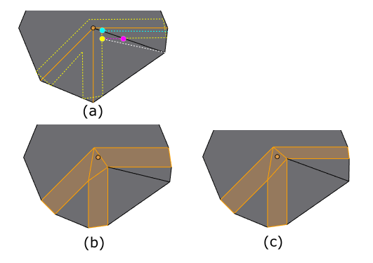
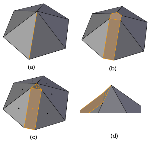
The harder case is when only some of the edges into a vertex are beveled. Consider this case, where in figure (a), the orange edges are beveled and the black ones are not.
In figure (a), the yellow dotted lines show where the beveled edge sides should go in order to make all bevels have the same width. As you can see, they do not meet at a common point on the unbeveled edge between two beveled edges. Since we need to keep that non-beveled edge, what can we do? Some choices:
- Allow Jogs: Let the two beveled edges on either side meet the non-beveled edges at different points. In the diagram (a), this would mean making the magenta and aqua vertices and joining them. Very ugly, and won't consider this option further.
- Preserve Widths: Keep the specified widths correct by changing the angle of the non-beveled edge. In the diagram (a), this would mean making the yellow vertex as the meeting point. The result is diagram (b). This could really distort the gross outline of the model but is not so bad if all of these edges are coplanar.
- Preserve Angles: Keep the angles of the non-beveled edges as they are by changing the widths of one of the bevels. In the diagram (a), this would mean choosing either the aqua point or the magenta point as the meeting point (or even some other point, such as the average of those two). The result in diagram (c) is when the aqua point is chosen. Note that the bevel amount for the horizontal beveled edge has now been adjusted and is different on each side of it: the top half is as it was before but the bottom half is now a lot narrower. One could also think of a variant where both sides are changed to the same value, but then that would force a cascade of changes all around the vertex, and would lead to further inconsistencies, so let us not pursue this variant.
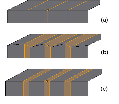
Blender used to use the Preserve Widths method. But this lead to unexpected behavior, reported as bugs by some artists. The issue is that you might expect that when there are unbeveled edges involved, they stay as they were and the new bevel edges slide along them (like in a loop slide operation):
You can see in the above that using Preserve Widths, shown in (b), looks pretty strange, even though the widths of the angled bevels (as measured perpendicularly across them) are even. Using Preserve Angles, shown in (c), is more likely what artists would like to see.
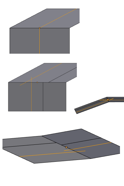
Another problem with Preserve Widths is that it is sometimes impossible to make a meeting point for the offset edges that gives the desired width on both edges. In the Bevel Ends - Not all Edges Beveled diagram above, the yellow point that is the intersection of the two offset lines looks like a point that can be used to preserve widths. However, that point only exists if, as in that diagram, everything is in the same plane. If the two beveled edges are in different planes, then the lines, in general will not meet:
In the above diagram, the orange lines show the needed offset lines to preserve widths. Those lines have been artificially extended in the three images below, shown from different viewpoints, to show that they do not meet at an intersection point. In such a case, one has to choose what to do, and falling back on Preserve Angles is probably the best of a number of not-great choices.
So now the method used by Blender is Preserve Angles, always, though the hook remains in the code to use Preserve Widths (only useful in planar cases), should we decide to offer that as a user option.
Update (July 5, 2015; for release version 2.76): due to user requests for the Preserve Widths behavior sometimes, we added a user option called Loop Slide (meaning: do the Preserve Angles behavior), on by default. Turning it off gives the Preserve Widths behavior.
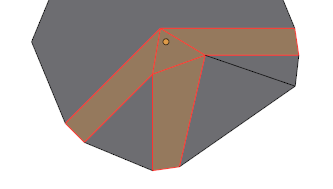
Using Preserve Angles has problems of its own: as soon as you start changing widths, you would like to change the widths at the other end of the edge to match, else you get an uneven effect like this:
In the above diagram, the mostly-vertical beveled edge has had its width changed at the center vertex in order to preserve angles, but the width at the bottom of that edge remains what the user specified. Clearly we should change the width at the bottom here to match the change made at the center. But notice that this means we cannot just process each vertex in isolation (as we are able to do if we use Preserve Widths, which makes no width changes). We could try to just change the width at the other end whenever we find we have to adjust a width, but what if that vertex has already been processed? E.g., in the above diagram, suppose we process all the vertices on the boundary before the middle one -- then we get the picture shown. We either need a more intelligent order of processing vertices, or we need a different algorithm that does a global width consistency pass before finally processing all the vertices.
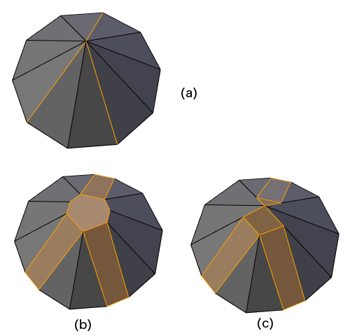
Another question that arises when only some edges into a vertex are beveled is illustrated by the following figure:
In the above figure, (a) shows a single edge out of six beveled. Whenever there are at least two unbeveled edges between beveled ones entering a vertex, we have a choice between these two options:
- Full Vertex Bevel: as shown in (b), make new vertices sliding along the unbeveled edges so as to make a vertex polygon to finish off the beveled edge(s)
- Partial Vertex Bevel: as shown in (c), and from another angle in detail in (d), leave the original vertex intact and only affect faces and edges adjacent to beveled edges. Sometimes the reflex face in (d) can look strange.
When you use Full Vertex Bevel, there is the question of how much to slide the new vertices along unbeveled edges. Blender currently uses the amount that the previously encountered beveled edge slid its vertex, which makes for an even-looking polygon.
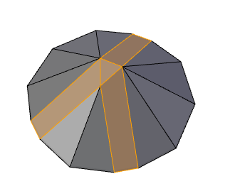
In general, there may be more than one group of beveled edges that need to get a vertex polygon, with each group separated by two or more unbeveled edges. E.g.:
For simplicity of code, and because the reflex face faces can look strange, Blender currently always uses the Full Vertex Bevel method. It is possible that artists might like Partial Vertex Bevel as an option.
Update (June 2, 2015, for Version 2.75): Users expressed a preference for the Partial Vertex Bevel algorithm in the case where there are 3 or more beveled edges (but not all edges beveled). So the code was updated to use that method. Now the three-out-of-ten edges case looks like:
When deciding where a vertex should go when there are several unbeveled edges attached to it, preference is given to sliding along an edge that isn't in the same plane as the adjacent edges over edges that are in the same plane. This preserves the silhouette of the original.
Multiple Segments
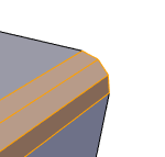
So far the discussion has been about bevels where each edge to be beveled turns into a single new face. Blender also allows for bevels with multiple segments, where a segment is a new face. For example, here is an edge that has been beveled into 3 segments:
Profile
The multiple segments should have parallel edges. Viewed end-on, the multisegment beveled edge has a profile, which is typically formed by evenly spacing the segments+1 vertices needed for the profile along a smooth curve:
What smooth curve should Blender use? In the above diagram, where there is a 90 degree angle between the faces adjacent to the beveled edge and the offsets along those faces are equal, the natural curve used is the quarter-circle arc with radius equal to the offset.
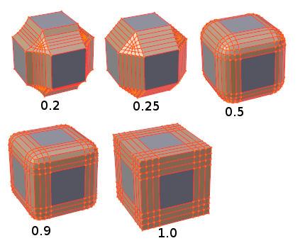
Artists have asked for more options for the profile, for instance to have concave profiles or have a profile that follows the original faces (but with multiple segments). One way to do this would be to use the parameterized family of Superellipses. Another option would be to allow an arbitrary Curve object to be specified as the profile. The 2.70 release of Blender implements the superellipse idea. There is now a profile parameter, which is really just 1/4 of the superellipse exponent:
Yet another thing to consider is the effect of running the subdivision algorithm on the result of a multisegment bevel. If you want the limit surface (as the number of subdivisions goes to infinity) to be, say, a circular arc, then the vertices should not be placed directly on a circular arc, but rather in different, further out, positions that could be calculated mathematically.
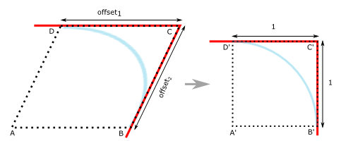
When the adjacent faces do not form a 90 degree angle, or the offsets along each face are different, then we need to distort the quarter-circle arc somehow.
The way to do this is shown in the above diagram. On the left, the edge to be beveled is at C, viewed end-on, and the desired offset distances along the adjacent faces (in red) are offset1 and offset2. Letter A is placed so as to make ABCD a parallelogram. Now we can make a transform matrix that maps ABCD onto A'B'C'D', a square with sides of length 1. Finally, we can place vertices evenly on the quarter-circle arc (in blue) in the unit square, and then use the inverse transform matrix to map them back onto the distorted quarter-circle arc in the original figure on the left.
Multiple Segment Corners
When all edges into a vertex are beveled into multiple segments, we need a way of making a vertex mesh which matches the profiles coming in and looks smooth.
Here are some choices for how to do that at a three-edge vertex.
For reference, let us give some names to the patterns in the above diagram:
- Poly - shown in (a), make a polygon out of the ends of the beveled edges; in general this polygon will be non-planar
- LatLng - shown in (b), the pattern is like the latitude and longitude lines on a globe
- None - shown in (c), there is no separate mesh for the vertex but rather the ends of the segments are joined up with their adjacent edge segments; this requires cutting the ends of the beveled edges in two halves
- Adj - shown in (d), the pattern shares quads between adjacent edges of the vertex polygon in a way that will be explained more below.
The Poly pattern is the one currently used for one-segment bevels. It is a good pattern if the beveled edges are all in one plane, so that the vertex polygon will be planar, but it does not look good in the non-planar, multi-segment case. Artists probably would prefer that the mesh around the vertex somehow continues the silhouette of the profiles of the beveled edges, when viewed from different angles. For a quarter-circle arc profile, this would lead to the natural choice of a one-eighth-sphere octant for the case where three beveled edges meet at 90 degree lines (as in the corner of a cube). Patterns (b) and (d) attempt to do that, putting a number of points on the sphere octant and joining them up into smaller polygons. The LatLng pattern is easy to compute, but it has several disadvantages: it is asymmetrical, requiring the choice of one vertex as the pole; it is not all quads, pinching into triangles at the pole; and it is hard to see how to generalize to cases with more than 3 beveled edges into a vertex. The Adj pattern has none of these disadvantages, and so Blender currently uses that in preference to LatLng. The None pattern gives a kind of sharp point that may be desired in special cases, but Blender currently only uses it in some cases where only two edges into a vertex are beveled (the code calls this a "weld").
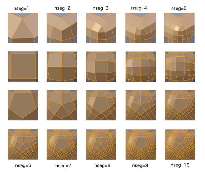
The Adj pattern is best described by showing some examples first:
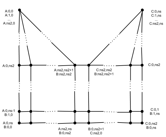
As you can see, the pattern is different for odd and even nseg (number of segments). For odd nsegs, there is a center polygon with the same number of sides as the number of beveled edges. For even nsegs, there is a single vertex in the center. The rule to create the pattern is:
- Form the boundary of the vertex mesh as in the Poly pattern (more on this below); the end of each beveled edge will have nseg segments and thus nseg+1 vertices across it (including the two ends). Call the group of vertices and edges that are on the profile of one beveled edge a boundary arc.
- Let ns2 be nseg /2, rounding down if nseg is odd. Then each boundary arc has ns2 rings of quads going from the previous boundary arc to the succeeding boundary arc. The tops and bottoms of the rings go from the last half of vertices of the preceding boundary arc to the first half of vertices of the succeeding boundary arc. The sides of the ring quads are the tops and bottoms for the ring quads of the preceding and succeeding boundary arcs.
- If nseg is odd, form a center polygon from the tops of the center quads in the innermost rings.
The above rules give the topology of the Adj pattern, but not how to set the coordinates of the vertices of the mesh. I have not been able to find a formula for placing the vertices on an octant of a sphere; it would be great if someone could find one. The current method used by Blender is described in the implementation section below. It can almost certainly be improved upon.
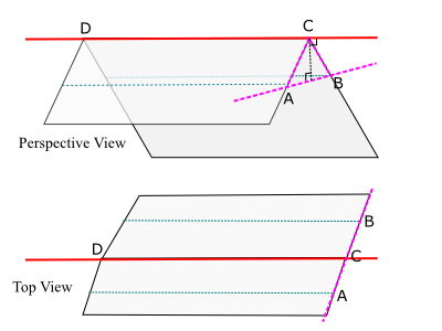
To make the boundary arcs for the Poly pattern and the outer rim of the Adj pattern, see the following diagram:
In the diagram, the bevel edge is part of the red line, and the offset lines are shown in dotted teal. Points A and B have been set as described in the Bevel Edge Ends section for the case of one segment. We need to find the position of point C. The diagram shows a natural choice, which is the point C on the beveled edge that is closest to line AB - that is, it makes a right angle with each of lines AB and CD. This forms a triangle ABC. Note that in general the plane containing ABC may be tilted, and not the plane that has the beveled edge as normal. Now that we have triangle ABC, we can form the parallelogram that extends it and transform to a unit square, as shown in the diagram Transform Non-Square Profile to Square Profile above. The quarter-circle arc can be divided into nseg equal pieces and used to place the internal vertices of the boundary arc in the unit square, and then transformed back into 3D space in their original positions.
The plane ABC is called the "profile" plane because it is the plane in which the multisegment profile (cross section end) is inscribed.
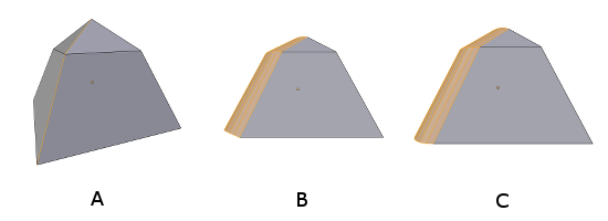
There are cases where the above method for defining the profile plane and center arc point C does not yield what artists expect. One example is when the edges to be beveled are as shown in (A) here:
The image in (B) shows the result of using the above algorithm to set the profile planes. Notice that the profile at the bottom lifts off the ground plane slightly, and the profile at the mid-level is also tilted out of the plane that contains all of the unbeveled horizontal edges at mid-level. The current Blender code recognizes these as special cases --- that is, when there are two unbeveled edges that either cross or terminate the beveled edge --- and adjusts the bevel plane to that of those unbeveled edges, as shown in (C).
Edge Bevel: Implementation
Data Structure for Vertex at End of Beveled Edge
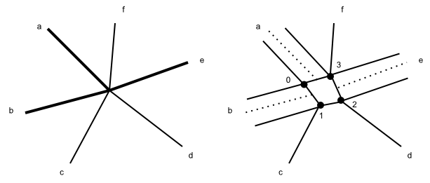
Consider a vertex that has a mixture of beveled and unbeveled edges leading into it.
On the left, the vertex in the middle is a vertex involved in a bevel,
and is represented by a BevVert struct, which contains
an array of EdgeHalf structs.
Each EdgeHalf represents, as its name implies, a half of an edge --
the half that is attached to this BevVert.
So in the example shown, the array has EdgeHalfs for edges a, b, c, d, e, and f.
In general, there is no intrinsic order to edges around a vertex:
think about a bunch of wire edges sticking out at all angles in space from a vertex.
But a very common case is that if you look down from the vertex normal,
all of the edges are connected to exactly two faces and you can find a counterclockwise
ordering of edges that is defined by going to the next edge by going across a common face.
The EdgeHalf array for a BevVert is arranged in that order
(starting from some arbitrary edge).
In the above diagram, if the vertex normal is coming out of the page, then a, b, c, d, e, f
would be a possible ordering in the array.
If there are gaps between some edges (no faces at all), the code tries to do the best it can
to order the subsequences that can be so ordered.
What happens after you bevel edges a, b, and e is that we create new vertices 0, 1, 2, and 3
as shown on the right. (Update: now we don't create separate vertices 1 and 2, but rather just a single one there
for the unbeveled edges to attach to.
In other words, we only create these vertices on either side of beveled edges, except for strange cases like only
a single edge beveled.)
These new vertices are called Boundary Vertices and are represented by a BoundVert struct.
The BoundVerts are linked together in a circular list, in counterclockwise order
(from the vertex normal side, the same as the edge order).
More than one EdgeHalf can be attached to the same BoundVert,
and an EdgeHalf that is for a beveled edge will be attached to two BoundVerts.
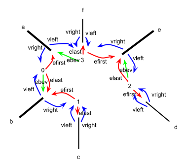
The following diagram shows some of the pointers that link the EdgeHalfs and
BoundVerts.
An EdgeHalf has a left side and a right side,
which are on the left and right sides of the edge when you look along the edge towards the BevVert
(from the vertex normal side).
The vleft and vright pointers of an EdgeHalf
point to the BoundVerts on its left and right side.
When the edge isn't beveled, they will both point to the same BoundVert,
but when it is beveled there will be two different BoundVerts.
For example, in the above diagram, beveled EdgeHalf b has
vleft = 0 and vright = 1.
Unbeveled edge d has vleft = vright = 2.
EdgeHalfs also have fprev and fnext
pointers which point to the faces between the edge and the previous and next edges, respectively,
in counterclockwise order. Those pointers may be NULL if there is no face between the edges.
A BoundVert has EdgeHalf pointers efirst and
elast, which point to the first and last EdgeHalfs in counterclockwise
order attached to the BoundVert.
If it is attached to the left side of a beveled edge then there will also be a ebev pointer that
points to that EdgeHalf.
For example, in the above diagram, BoundVert 2 has efirst = d,
elast = ebev = 3.
The vertex mesh for a BevVert is kept in a VMesh struct.
The main component of that is an array of NewVert structs, each of which
holds a 3D coordinate and, eventually, the BMesh vertex instantiated for it.
The NewVerts are indexed in the array according to the mesh pattern.
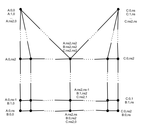
For the Adj pattern, they are indexed by (i, j, k) where i is the index of the BoundVert,
j is the index of the ring, and k is the index of the segment along a boundary arc between the
given BoundVert and its counterclockwise successor.
The vertices in the pattern have two or more indices according to this scheme.
Of course there should only be one BMVert allocated for a vertex,
so some of the NewVerts will share a BMesh vertex.
The above two diagrams show the indexing patterns for an even and odd number of segments, and three vertices in order, A, B, and C. In the diagrams, it is assumed that the predecessor boundary arc to A and the successor boundary arc to C are not for beveled edges. When a boundary arc is not for a beveled edge then only segment indices 0 and nseg are used.
Update: Now even boundary arcs for non-beveled edges are divided into nseg segments. This yields a generally more pleasing vertex mesh, and is also what is needed for multisegment vertex bevel. The downside is that now the adjacent old faces will be higher-degree ngons when rebuild; but they should be flat so maybe this isn't such a big downside. Leaving the above diagrams there in case some future developer wants to try going back to the mixed mode of boundary arcs.
Calculating Vertex Positions for Adj Vertex Mesh Pattern
The original method for calculating the vertex positions for the Adj vertex mesh pattern was:
- Calculate the position of the boundary arc vertices using the triangle formed by the two end vertices and the closest point on the beveled edge to the line between them, as described above in the Multiple Segment Corners section.
- For the inner rings of a given boundary arc, use the same method: find the endpoints on the adjacent boundary arcs and then form the triangle with those two points and the closest point on the beveled edge, and use the map-to-unit-square method to map a quarter-circle arc into position.
- Now there will be several choices for each vertex, because they can be indexed in more than one way (see the previous section), due to being on a ring for more than one boundary arc. Solve this dilemma by averaging the coordinate positions of all aliased indices for a vertex.
While this produced results that looked OK in many cases, there were also a lot of cases where it didn't work well. For instance, for some corner angles, as the number of segments increased, the contour lines looked uneven and could even cross. Also, this method did not seem to converge to a solution where the vertex mesh smoothly transitioned into the adjacent sides (in other words, the normals of the planes at the edges of the vertex mesh didn't converge to the normals of the adjacent sides).
For these reasons, the literature was consulted for a better solution. Here are papers about two similar approaches:
- N-Sided Hole Filling and Vertex Blending Using Subdivision Surfaces, by Wei-Chung Hwang and Jung-Hong Chuang. Journal of Information Science and Engineering 19, 857-879 (2003).
- Filling N-Sided Holes Using Combined Subdivision Schemes, by Adi Levin. International Conference on Curves and Surfaces [4th], Saint-Malo, France, July 1999.
Both use the 'Adj' pattern, and use subdivision schemes with modification in order to match the boundary curves and the tangencies there. The Hwang/Chuang paper uses a quadratric subdivision (like Doo-Sabin), while the Levin paper uses cubic subdivision (like Catmull-Clark).
After implementing both, I ended up choosing to use the Levin method.
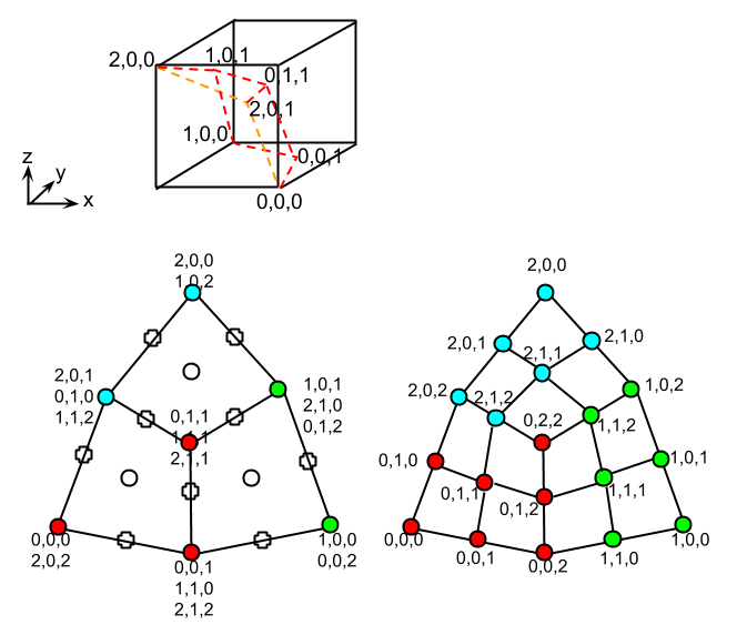
A key part of the Levin method is to do a Catmull-Clark subdivision step. He recommends a variant that uses weights calculated by Sabin. As a concrete example of our indexing scheme, here is a picture of indexing of the unit cube with BoundVerts at (1,0,0), (0,1,0), and (0,0,1) and quarter-circle arcs on the faces of orthogonal planes through the origin:
The mesh on the left in the above diagram shows how the initial construction works:
each boundary arc is divided in two, and one central vertex is made to join to the middle vertices.
The coordinates of the middle vertex are up to the designer.
We move it along the direction from the original vertex to the centroid of the boundary vertices.
The amount to move depends on the profile parameter.
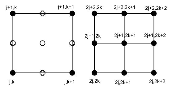
For the general formulas, here is one step of a an internal quad turning into four quads with one step:
Let M be the mesh on the left and M’ be the mesh on the right. M' is formed by adding new edges-vertices (crosses) and a new face-vertex (circle). Also, the coordinates of the old vertices(vertex-vertices) are changed. The Catmull-Clark rules give the following. Assume we make all the face vertices first, then all the edge ones, then all the vertex ones.
New face vertex M’(2j+1, 2k+1):
| f(j,k) | = avg(M(j,k) + M(j,k+1) + M(j+1,k) + M(j+1,k+1)) |
Note that f(j,k) is stored in M’(2j+1, 2k+1), which will be used below.
New vertical edge vertex M’(2j+1,2k):
| ev(j,k) | = avg(M(j,k) + M(j+1,k) + f(j,k-1) + f(j,k)) |
| = avg(M(j,k) + M(j+1,k) + M’(2j+1,2(k-1)+1) + M’(2j+1,2k+1)) |
New horizontal edge vertex M’(2j,2k+1):
| eh(j,k) | = avg(M(j,k) + M(j,k+1) + f(j-1,k) + f(j,k)) |
| = avg(M(j,k) + M(j,k+1) + M’(2(j-1)+1,2k+1) + M’(2j+1,2k+1)) |
New vertex vertex M’(2j,2k):
| v(j,k) | = α(4) * avg(ev(j-1,k) + ev(j,k) + eh(j,k-1) + eh(j,k)) |
| + β(4) * avg(f(j-1,k-1) + f(j,k-1) + f(j-1,k) + f(j,k)) + γ(4) * M(j,k) | |
| = α(4) * avg(M’(2(j-1)+1,2k) + M’(2j+1,2k) + M’(2j,2(k-1)+1) + M’(2j,2k+1)) | |
| + β(4) * avg(M’(2(j-1)+1,2(k-1)+1) + M’(2j+1,2(k-1)+1) + M’(2(j-1)+1,2k+1) | |
| + M’(2j+1,2k+1)) + γ(4) * M(j,k) |
See the paper or the code for the weight functions α(), β(), and γ().
There is also the new center vertex which is like the New vertex vertex formula but needs to gather new edge vertices and new face vertices all around it, and combine it with α, β, γ that depend on the number of sides of the hole.
Finally, the border and corner vertices need special adjustment. I implemented the formulas in the paper and they didn't seem to work. They seemed too extreme and not convergent to the desired boundary curves. Furthermore, reading Levin's thesis, which describes the same process, it appears the formulas are different. I probably am misunderstanding, but it is also possible there is an error in one or the other.
Instead, what I did is resample the boundary curves at even parameter spacing and set them to that.
Now there are two problems with the above method that still need to be resolved:
- As you iterate, you always double the number of segments. So you will only get powers of 2 for the number of segments. We need to have an arbitrary number of segments.
- The spacing between the lines does not come out even (except where forced by resampling at the boundary).
Two solve these problems, the adj_vmesh() subdivides until the power of 2 exceeds the desired number of segments, and then uses interp_vmesh() to sample the required number of segments at even intervals along two dimensions.
Even Sampling of Superellipses
The introduction of profile control via the superellipse parameter brought a new problem to the implementation: how to sample the profile so that you get evenly spaced chords.
With a circular arc for the profile, it is easy, using the trigonometric parameterization of the unit circle:
P(Θ) = (cos Θ, sin Θ)
gives the P = (x, y) coordinates for points on the arc as a function of the angle Θ. This has the nice property that if you divide a quarter circle angle into n equal pieces, and feed the cumulative angles into the above formula, then the arc lengths (and chord lengths) will all be equal. This is what an artist would expect along a boundary curve.
Unfortunately, the same doesn't hold for the trigonometric parameterization of a superellipse:
P(Θ) = (cos2/r Θ, sin2/r Θ)
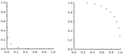
when sampled at even intervals of Θ, gives an uneven spacing of arc length or chord length, when r is not equal to 2. The following picture shows this:
On the left is a superellipse with parameter r=0.3, and on the right is one with parameter r=3.0. The dots show the points along the arc using even spacing of Θ. For parameters < 2, the dots bunch together near the ends; for parameters > 2, the dots bunch together in the middle.
There are two other ways of parameterizing superellipses. The angle-center parameterization is:
P(Θ) = (R cos Θ, R sin Θ) where R = (cosr Θ + sinr Θ)-1/r
And there's the explicit equation for y in terms of x:
y = (1 - xr)1/r
I'll spare you the graphs, but they show that neither of these parameterizations yield an even spacing of the dots for an even spacing of the parameter. In fact, a search of the literature failed to find a closed form parameterization of a superellipse that would give an even spacing.
Ideally, we would like, for a given nseg and superellipse parameter r, to find a way of getting the ith (x, y) point along the quarter arc in the first quadrant, where i varies from Θ to nseg, such that the chord lengths between successive points are all equal.
The code does this by precomputing a series of Θ values such that evaluating at each of them in turn yields equal-length chords. (Actually, it precalculates a series of a parameter u that is a scaled version of Θ that avoids dealing with π so much.) It currently implements this as follows:
- The function
superellipse_co(u, r, r_co)evaluates the trigonometric parameterization of the superellipse with parameter r at u = Θ/4 (so as u goes from 0 to 2, the arc traverses the first quadrant). - The function
find_superellipse_chord_u(u0, d2goal, r)finds a value of u > u0 so that the square of the chord length from the point at u0 to the point at u equals d2goal. It works by binary search on suitable u, until the chord length squareds match to suitable tolerance. - The function
find_even_superellipse_params(n, r, r_params)finds and returns an array of u parameters to give n even chords in the first quadrant. It does this by binary searching for the chord length squared that makes when repeated n times goes from the beginning to the end of the quadrant. Thefind_superellipse_chord_ufunction is used as a helper in this binary search.
For a given invocation of Bevel, which has a particular nseg, we need to precalculate the superellipse u's for that nseg. Also, because we need to do superellipse sampling during the Catmull-Clark subdivision steps, we also need to precalculate the u's for all n that are powers of 2 up to a value that equals or exceeds nseg. While this may not be exactly right, we just do this for the highest power of 2 needed, and then when we need the intervals for a power of 2 less than that, we suitably subsample the values for the highest power of two.
Consistent Widths for Even Bevels
To show the problem of choosing consistent edge widths, consider the following diagram:
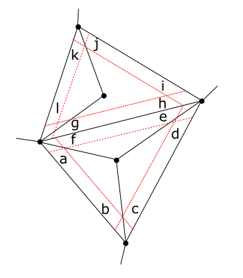
In the diagram above, the black dots and lines are vertices and edges of a mesh, and the dotted red lines show where we would like to move the offset edges if beveling all of the edges of the two larger triangles but not beveling the edges joining to the center dots. Notice that some of the red lines happen to meet on the spoke edges, or at least come close, but in general they do not, and if we want to preserve angles, we will have to adjust some bevel widths. The letters in the diagrams label widths (between a black line and a dotted red line). A beveled edge might be forced to have four different widths: on each side and each end. For example, e, f, g, and h widths might all have to be different in the general case. (There are also widths on the other sides of the outer beveled edges too, not shown in this diagram.)
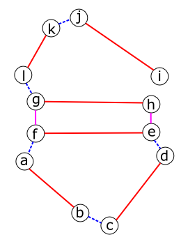
We can make a graph showing which widths are dependent on other widths:
In the above diagram, the red lines connect widths that are part of the same bevel edge side. The magenta lines connect widths that are part of the same bevel edge end (on opposite sides of the original edge). And the blue dotted lines connect widths that are on beveled edges separated by one unbeveled edge. We would like the widths connected by red lines to be the same, so that you don't get the tapered-edge effect on beveled edges. We would like the widths connected by magenta lines to be the same so that the new bevel face evenly straddles the original edge. We are forced to make the edges connected by dotted blue lines to be related according to a function of the angles involved (really: so that the meet point is somewhere sliding along the unbeveled intermediate edge). You can see that because there are cycles in the graph, it may not be possible to satisfy all the constraints; there may be situations in which we will have to accept some tapered beveled edges. But by using the graph to adjust the edges in a certain order, we can minimize the number of places where that needs to happen, and in many cases eliminate the need for that to happen. Note: the condition that widths connected by magenta lines should be equal is probably not very important. What matters more is that the final new bevel face looks even - the memory of how it straddled the original face is probably gone. An alternate desired constraint might be that the sum of the widths connected by magenta lines should be as close as possible to the width originally specified by the user.
What can we do when there are conflicts? Consider this diagram:
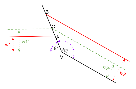
The desired offsets for the two beveled edges are w1 and w2, which would like us to put the vertex at A and B respectively. We are going to have to pick some C at or between A and B at which to compromise; this will lead to new offsets w1’ and w2’. We would like to minimize either |w1 - w1’| + |w2 - w2’|, or (w1 - w1’)2 + (w2 - w2’)2. Let δ = the distance between A and B. We want to choose a λ between 0 and 1 and place C a distance λδ from A along the line AB. So to minimize the sum of absolute values, we minimize:
λδ sin θ1 - (1-λ)δ sin θ2 = δ(λ sin θ1 - (1-λ) sin θ2)
which is minimized at λ = sin θ2 / (sin θ1 + sin θ2)
To minimize the sum of squares, we minimize
δ2(λ2 sin2 θ1 + (1-λ)2 sin2 θ2)
which is minimized (using derivatives) at sin2 θ2 / (sin2 θ1 + sin2 θ2)
The diagram also illustrates that there are going to be some special cases. If both θs are zero (so all three lines are the same), then can only have all widths be zero. If either θ is straight or reflex then there is no way for any offset line to meet the unbeveled edge; in that case we need to use the ‘offset-in-two-planes’ method to set coordinate C (and that method might fail because the lines don’t meet, and if so, we can’t fall back to the ‘on-edge’ method! need to just choose something like the average of the closes points on each line).
Update: The method first implemented (trying to match widths as we go, followed by a depth-first search to adjust as much as possible) did not work all that well. The non-determinism (or, at least, dependence on initial vertex order) meant that different parts of the model could get different widths even though they are topologically the same. So we are now going with a different method, detailed here.
The approach is to solve a least squares problem. Let each edge ei have widths Li and Ri. Then when we are sliding along a non-beveled edge between beveled edges, as in the diagram above, the variable Li depends on Rj according to this formula:
Li = Rj (sin θ1 / sin θ2) = gi Ri where gi = sin θ1 / sin θ2
where R is w'2 in the above diagram.
An important simplifying observation is that if we ignore the magenta lines in the dependency graph above (as we argued we likely could), then the dependencies are much simplified: they will always be the disjoint union of a number of chains (straight line dependencies) and cycles. So we only have to figure out how to solve the least squares problem for chains and cycles - and then we can solve each independently.
Solving a Chain
Suppose we have a chain of 4 vertices where with 3 beveled edges joining them, and a slide happening at all 4 vertices (we consider only one side of the chain in this derivation). Then the least squares problem we want to solve can be expressed with two matrices:
A 1 -g1 0 0 0 1 -g2 0 0 0 1 -1 w 0 0 0 0 w 0 0 0 0 w 0 0 0 0 w
b 0 0 0 w R0 w R1 w R2 w L3
These go with a parameter column vector x = {r0, r1, r2, l3} -- that is, the right width (the width on the right of the edge at the end where you are looking at a vertex) for the first three parameters and the left width for the edge just beyond the end of the chain. The other left edges are dependent on the preceding edge's right width. E.g., l1 = g1 r1. The equation
A x = b
expresses what we would like to be true: the first three rows say that the difference between the right and end left end of an edge is zero. Call these the even width constraints. Note that the edge just before the chain and just after it do not have even width constraints because we are free to set their other ends to the value at the end on the chain. The last four rows are match spec constraints. They say that the width ri should match the specification for that edge, Ri. We multiply each of those rows by w so that we can make those constraints more or less important than the even width constraints.
Note that we have 7 equations but only 4 variables. So in general we can't make them all true, meaning we can't both have even widths and matching specs -- we will have to compromise. Whatever x we choose will leave a residual vector, r = b - Ax. The problem of minimizing the 2-norm of that vector is called a linear least squares problem. There is a package, Eigen3, linked with Blender, that can solve such problems, given matrices A and b. There is also another package, Ceres, linked with Blender which can solve non-linear least squares problems, which allows more general residuals than the linear equation form shown here, and also allows one to set upper and lower bounds on the parameters; I found that using Ceres instead of Eigen3 for this problem was about twice as slow, so the current implementation uses Eigen3. However, even using Eigen3 to solve these problems is fairly expensive compared to all of the rest of bevel calculations. For an example, a mesh with 4 chains of 210 edges each took 0.08 seconds to bevel, of which .055 seconds was just this least squares problem. We want bevel to be fast enough that it seems instantaneous to a user, so they can smoothly adjust the width interactively. For this reason, we will pursue a faster method.
The linear least squares problem has an exact solution, found by solving ATAx = ATb. This is essentially what the Eigen3 routine solves. Our A matrix has a special form that is quite sparse, and it turns out that ATA is also quite sparse. But the inverse matrix (ATA)-1 is not. And the pattern of entries in that inverse is not easy to describe. So there isn't an easy way to code up the exact solution -- we might as well continue to use Eigen3, which uses sparse matrix methods.
However, the even width constraints have a form that yields an easy-to-code solution by backsubstitution to express each parameter in terms of the last one, which we can regard as the one degree of freedom we have in solving the n-1 even width constraints for n variables. So, rather than solve the above system, which gives a way of soft combining the desire to match widths with some (possibly more or less weighted) desire to match specs, we can pursue a two-part solution: first solve the equal width constraints exactly, in terms of the final parameter. Then express the equal specs constraints in terms of that parameter. It will be a quadratic equation in one variable, which is easy to minimize. This doesn't have the same tradeoff ability as the weighted solution, but will be a lot faster to execute (a linear running-time solution instead of a quadratic or approximate iterative one).
This two-part solution has this derivation. First, solving for parameters (number 1 to n), the parameter values take this form:
pn = a (for some free variable a)
and
pi = gi gi+1 gi+2 ... gn-1 a
for i < n, assuming gn-1 is defined as 1. Call that product Gi, and let Gn = 1.
Now the match specs part least squares error equations can be written
(G1 a - s1)2 + ... + (Gn a - sn)2
where si is the specification width for parameter i. Expanding out the squaring:
Σi=1n (Gi2 a2 - 2 Gisi a + si2)
which we can minimize by taking the derivative with respect to a and setting to zero:
Σi=1n (2 Gi2 a - 2 Gisi) = 0
which is solved as
a = Σi=1n si / Σi=1n Gi
How well does this two-step calculation do compared to the weighted one? Well, it is faster. For the 4 x 210 chain example cited above, the total time to do this width adjustment drops from .055 seconds to .005 seconds, and now represents 14% of the total bevel time instead of 69%. What about the quality?
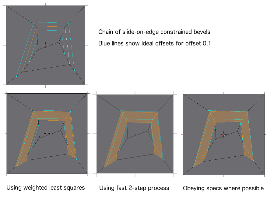
The above diagram shows on the top the positions of where the offset edges should go to make the widths exactly as specified. As you can see, forcing the meeting point to be on the existing edges means that we cannot simultaneously get the ideal widths on all edges. On the bottom row, the leftmost picture shows the result of using the full least squares solution, with spec matching weighted at 0.2. The middle shows the result of using the faster 2-step process just derived. The final picture shows what happens if we try to match the specs (it is impossible to do that in the middle because we have to compromise between the two desired widths, but it is possible to make the free ends match exactly -- note how that makes the bevels taper.
In the end, different artists may want different results, but for now we will assume that the result in the second diagram is OK with artists. The first result may be slightly preferred by some -- at a cost of a 2% difference in widths at the two ends, the weighted least squares solution finds a solution where the maximum deviation from spec width is 38% instead of the 50% deviation achieved by the faster process.
Solving a Cycle
The A matrix for the cycle case is almost the same as the chain. The difference is that for n edges there will be n even width rows:
A 1 -g1 0 0 0 1 -g2 0 0 0 1 -g3 -g4 0 0 1 w 0 0 0 0 w 0 0 0 0 w 0 0 0 0 w
Here it seems we don't get the same 1 degree of freedom in solving the even width constraints -- there would seem to be only one solution (and it will be achieved by setting all parameters to zero -- not very interesting!). But there is an exception. The determinant of the first n rows is zero when the product g1 g2 ... gn = 1. That can happen surprisingly often with models that artists build. For instance, if all the sliding edges are bisectors of their angles, then the same point on the sliding edge will work for both edges attached there (this is the case where all the sin rations, gi are 1). Other cases occur when the model has some symmetry, so that for every pair θ1, θ2 one later encounters a matching θ2, θ1 in the cycle. Then the sin ratios are inverses of each other, and so cancel out to 1 when multiplying. So it seems worthwhile to derive the fast case for cycles when that product is 1.
When the product of the g's is 1, then we get back one degree of freedom, and we can again express all of widths in terms of the g's and the free variable that is the last parameter (some arbitrary last element in the way the cycle is discovered). The formula for solution turns out to be the same as for the chain case, just that the final couple of g's can have values different from 1. A similar statement is true about the second step, minimizing the spec deviations in terms of the one free variable of the first part.
Good UV Interpolation
One of the hidden trickier aspects of beveling involves how to properly assign various auxiliary data to newly created vertices, edges, and faces: that is, things like weights, creases, colors, and UV values. Of these, getting the UV values right turned out to be by far the trickiest.
UV values give a mapping from corners of faces in 3D into 2D coordinates in a UV map (usually used for mapping textures). Inside Blender, the concept of a face corner is called a Loop -- it contains a vertex, and outgoing edge, and various custom data layers, among which are UV values (there can be more than one UV layer). Note that there are multiple loops at the same vertex -- one per face touching that vertex. Thus, there will be multiple UV values at the vertex. This means that it is possible, and indeed usually necessary, for there to be discontinuities in the UV mapping at some vertices. For example, if an edge is marked as a seam and then the object is unfolded to map a UV map, one or both of the vertices of that edge will likely appear several places in the UV map.
Now the general method used inside Blender to assign Custom Data values, like UVs, to newly created target loops is to use loop interpolation in some source face. The way that works is that the source face is flattened into a plane polygon, and then vertex position of the target loop is projected into the same plane. Finally, an interpolation algorithm is used to interpolate each of the custom data points from the values of those same data points at each of the loops of the source face (see Generalized Barycentric Coordinates on Irregular Polygons by Meyer, Lee, Barr, and Desbrun for the algorithm).
Now for most kinds of Custom Data, it is easy: when you create a new face, you go through each vertex in the face, find the closest original (before beveling) face, and interpolate in that.
But this doesn't always work well for UVs, for two reasons:
- If the new face straddles an edge of the original object, so that the closest original face is not the same for all vertices of the new face, then mapped face in UV space will also straddle original mapped faces. Usually this is fine, and what is desired, but if the straddled edge is a seam then the new mapped UV face will likely cross a no mans land in UV space, where either nothing was mapped before or maybe another UV island is mapped. The latter is worse, but in either case, the original texture may now be outside the lines of the original UV net, and so you may get black textures until the user does some UV or texture image editing. We'd prefer that you not have to do this after doing a bevel.
- If the new face has vertices that are notionally on one of the original edges, and there's another new face sharing those vertices, we would like the UV net post-bevel to be connected there. The interpolation method makes sure that this is true if the vertices are actually on the edge; but sometimes they are above the edge, and the projection into the faces on either side of the edge leads to different interpolations, and thus, an unconnected net.
To solve the first of these problems, we do a careful analysis of new faces that straddle edges to see if it is OK to have different vertices interpolated in different faces without causing the no mans land problem. If it is not OK, then one face is picked and all edges are interpolated in it. But even in this latter case there is work to do to avoid no mans land: we need to snap the vertices that are outside the interpolating face to edges of that face.
To solve the second problem, we do an analysis of new vertices to see which ones are nominally on original edges (but may in fact be in space over the edges). Then we temporarily snap those vertices to the edges while interpolating, and then put them back where they belong.
There is a single bev_create_ngon function that all face creation goes through in the bevel tool.
It takes in the array of vertices to make a face from, and it also takes in two parallel arrays to control interpolation: one is an array of faces to interpolate in, the other is an array of edges to snap to (temporarily) while interpolating. If all interpolation is in the same face then there is a separate argument for that, and the face array can be NULL.
There is also some code that explicitly merges all the UVs around a given vertex, using the average values. This is called in cases where it is known that all the faces connected to that vertex should be connected in UV space. (This is legacy code, and I'm not sure that these merge-UV routines are still needed -- it could be that the later-added edge-snapping capability has ensured that whenever this is called, the interpolated values of all loops will be the same anyway.)
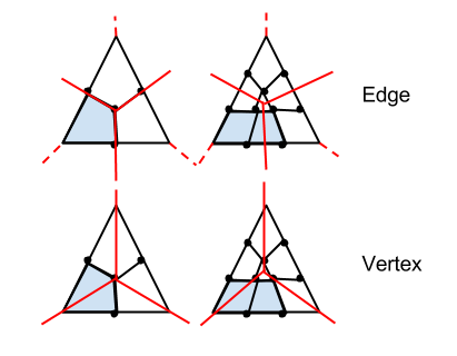
To see an example of the analysis that was done for the vertex meshes, consider this diagram:
In these diagrams, the solid red lines show the original model edges. For edge bevels, the dotted red lines show the newly created edges for the outside edges of the edge bevels. For vertex bevels, the solid red lines continue as is from the vertex mesh.
Recall the number scheme for the vertices of the vertex mesh. If we have n sides, and ns/2 = nsegments/2 (truncating division), then there are n boundary vertices, and all of the vertex mesh vertices are numbered (i, j, k) where i is the boundary vertex index, j is the ring index, and k is the index along the side.
We can find a representative face for each boundary vertex, meaning the face that we should do interpolation in for that boundary vertex. For edge bevels, you can see that the boundary vertices are totally within one of the faces between beveled edges, so that is the representative face. For vertex bevels, the boundary vertices are on original edges, so the could get either the previous (in CCW order) or next face as the representative face; we arbitrarily choose the previous face.
We make these canonical quads: (i,j,k), (i,j,k+1), (i,j+1,k+1), (i,j+1,k)
where i in [0,n-1]; j in [0,ns/2-1], and k in [0,ns/2-1+odd] (odd is 1 if there are an odd number of segments).
For this quad, here is the analysis of what arguments to give to bev_create_ngon:
- Edge bevel, even nsegments
- Use the representative face for boundary vertex i for all four vertices of the quad
- When k = ns/2 - 1, snap the 2nd and 3rd vertices to the side's beveled edge
- When j = ns/2 - 1, snap the 3rd and 4th vertices to the previous (CCW) side's beveled edge (break tie in favor of previous case)
- Edge bevel, odd nsegments
- Usually use the representative face for boundary vertex i for all four vertices of the quad. However, if k=ns/2 and the side's beveled edge is not a seam, then it is OK to use the representative face for boundary vertex i+1 for the 2nd and 3rd vertices.
- When "k" = ns/2, snap the 2nd and 3rd vertices to the side's beveled edge
- Vertex bevel, j = k
- If the on edge for boundary vertex i is a seam, then use the representative face for all four vertices. Otherwise, use that for the 1st, 3rd, and 4th vertices, but use the representative face of boundary vertex "i"+1 for the 2nd vertex
- Snap the 1st and 3rd vertices to the on edge. But the k=ns/2 and j'==ns/2-1 case is exceptional: we use boundary edge i to snap the 4th vertex and boundary edge i+1 to snap the 3rd vertex
- Vertex bevel, j < k
- Use the i+1 representative face for all vertices. No edge snapping.
- Vertex bevel, j > k
- Use the i representative face for all vertices. No edge snapping.
Besides the polygons made for vertex meshes, there are two other classes of polygons made by the bevel tool. One class is the edge polygons, made only for edge bevels. These are the long thing faces that replace the original beveled edge. There will be nsegments such polygons, side-by-side, for each beveled edge. The only edge polygons that need special treatment are those that touch the center line (for even nsegments) or those that straddle it (for odd nsegments). The analysis is similar to what we showed for the vertex mesh cases, so we will omit the details here. In order to keep the UV net as connected as desired, there is some code to see what happens where the edge polygons butt up against the vertex meshes (or other edge meshes, in the case of welds), and sometimes do a merge UVs around vertices there.
The other class is the replacement face polygons: that is, all the original faces of the model that touch a beveled vertex or edge, and thus have to be remade using the moved / added vertices from the vertex mesh and edge polygons. Nothing special needs to be done as far as interpolation for these -- they just get interpolated in the corresponding original face, and no snapping is needed.
